Modern Evolutionary Biology

I. Population Genetics

A. Overview

Sources of Variation                                                Agents of Change
MUTATION:
-New Genes:                                                           Natural Selection
     point mutation                                                    Mutation (polyploidy can make new species)  

RECOMBINATION:
- New Genes:
    exon shuffling
-New Genotypes:
    -crossing over
    - independent assortment

In the early 20th century, at the same time that T. H. Morgan was studying mutations and creating linkage maps, other biologists were considering the evolutionary implications of this new knowledge regarding genetic variation. They appreciated that individuals do not evolve - evolution is a process that occurs at the population level. For example, as a consequence of differential reproductive success among individuals in a population, the range of phenotypes and their relative frequencies in the population will change over time. Individuals are born, life, reproduce (maybe) and die. As a result of passing on their genes at different frequencies, the genetic structure of the population changes over time (evolution). Two biologists, G. Hardy and W. Weinberg, constructed a model to explain how the genetic structure of a population might change over time.

Their model begins by constructing an 'equilibrium' model - a model of what the genetic structure would look like, and how it would behave, if there was NO CHANGE over time. (We can liken this to a "statistical null hypothesis of no effect"). Then, an actual population is compared to this model, to see whether the population is evolving or not.    

B. The Genetic Structure of a Population

Our first step is to describe the genetic structure of a population; we need to do this before we can model what it would do over time. The genetic structure of a population is defined by the gene array and the genotypic array. To understand what these are, some definitions are necessary: 

1. Definitions:

                - Evolution: a change in the genetic structure of a population
                - Population: a group of interbreeding organisms that share a common gene pool; spatiotemporally and genetically defined
                - Gene Pool:  sum total of alleles held by individuals in a population
                - Genetic structure: Gene array and Genotypic array
                - Gene/Allele Frequency: % of alleles at a locus of a particular type
                - Gene Array: % of all alleles at a locus: must sum to 1.
                - Genotypic Frequency: % of individuals with a particular genotype
                - Genotypic Array: % of all genotypes for loci considered; must = 1.          

2. Basic Computations - Determining the Genotypic and Gene Arrays:

The easiest way to understand what these definitions represent is to work a problem showing how they are computed.               

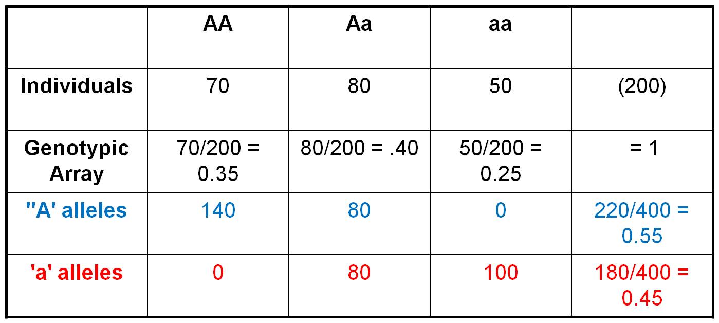
Consider the population shown to the right, in which there are 70 AA individuals, 80 heterozygotes, and 50 aa individuals. We can easily calculate the Genotypic Frequencies by dividing each of these values by the total number of individuals in the population. So, the Genotypic Frequency of AA = 70/200 = 0.35. If we account for all individuals in the population (and haven't made any careless math errors), then the three genotypic frequencies should sum to 1.0. The Genotypic Array would list all three genotypic frequencies: f(AA) = 0.35, f(Aa) = 0.40, f(aa) = 0.25. A Gene Frequency is the % of all genes in a population of a given type. This can be calculated two ways. First, let's do it the most obvious and direct way, by counting the alleles carried by each individual. So, there are 70 AA individuals. Each carries 2 'A' alleles, so collectively they are 'carrying' 140 'A' alleles. The 80 heterozygotes are each carrying 1 'A' allele. And of course, the 'aa' individuals aren't carrying any 'A' alleles. So, in total, there are 220 'A' alleles in the population. With 200 diploid individuals, there are a total of 400 alleles at this locus. So, the gene frequency of the 'A' gene = f(A) = 220/400 = 0.55. We can calculate the frequency of the 'a' alleles the same way. The 50 'aa' individuals are carrying 2 'a' alleles each, for a total of 100 'a' alleles. The 80 heterozygotes are each carrying an 'a' allele, and the 140 AA homozygotes aren't carrying any 'a' alleles. So, in total, there are 180 'a' alleles out of a total of 400, for a gene frequency f(a) = 180/400 = 0.45. The gene array presents all the gene frequencies, as: f(A) = 0.55, f(a) = 0.45.

There is a faster way to calculate the gene frequencies in a population than adding up the genes contributed by each genotype. Rather, you can use these handy formulae:

f(A) = f(AA) + f(Aa)/2

f(a) = f(aa) + f(Aa)/2

So, to calculate the frequency of a gene in a population, you add the frequency of homozygotes for that allele with 1/2 the frequency of heterozygotes. In our example, this would be:

f(A) = 0.35 + 0.4/2 = 0.35 + 0.2 = 0.55

f(a) = 0.25 + 0.4/2 = 0.25 + 0.2 = 0.45

Wow... that's a lot faster.

C. The Hardy-Weinberg Equilibrium Model

1. Goal:

The goal of the "Hardy-Weinberg Equilibrium Model" (HWE) is to describe what the genetic structure of the population would be if NO evolutionary change occurs. Working independently, Hardy and Weinberg realized that the gene frequencies in a population will NOT change - will remain in EQUILIBRIUM - if the following conditions are met:

- there is random mating

- no selection

- no mutation

- no migration

- and the population is infinitely large.

And, they realized that a population will reach an equilibrium in GENOTYPIC frequencies, too, after one generation of meeting these expectations. And, for as long as these conditions are met, a population will NOT EVOLVE. Let's see how they came by these conditions.

2. Example:

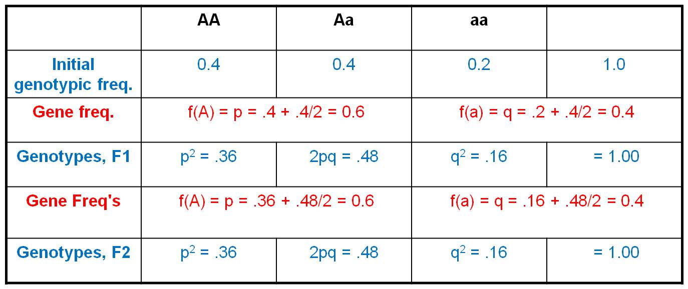
Consider an initial population, with a genotypic array as shown. The gene frequencies are:   

A = 0.4 + (0.4/2) = 0.6

a = 0.2 + (0.4/2) = 0.4                

Now, consider this gene pool in which 60% of the alleles are 'A' and 40% of the alleles are 'a' (as defined by the gene frequencies). The gene frequencies represent the frequencies of gametes carrying these gens; so 60% of sperm are 'A', 40% are 'a', and likewsie for eggs.

So, now we employ the HWE model. IF the population mates at random, then we can use the product rule to determine the probability of any two gametes coming together. The propability that and 'A' sperm fertilizes an 'A' egg = 0.6 x 0.6 = 0.36. And of course, this is the only way to produce an 'AA' zygote. The frequency of 'AA' zygotes (the F1 offspring) produced by this population should be 0.36. Likewise, the probability that an 'a' sperm fertilizes an 'a' egg = 0.4 x 0.4 = 0.16. And again, this is the only way to make an 'aa' zygote, so the total frequency of 'aa' zygotes in the F1 will be 0.16. Now, there are two ways to make an 'Aa' zygote: an 'A' sperm can fertilize an 'a' egg (probability = 0.6 x 0.4 = 0.24), and an 'a' sperm can fertilize an 'A' egg (also with a probability of 0.4 x 0.6 = 0.24). So, the total frequency of Aa zygotes in the F1 will be 2 x 0.24 = 0.48. If we generalize, and let f(A) = p and f(a) = q, then the genotypic frequencies under HWE can be calculated as: f(AA) = p², f(Aa) = 2pq, and f(aa) = q².

What is the genetic structure of the population in the F1? Well, f(A) = f(AA) + f(Aa)/2 = 0.36 + 0.48/2 = 0.36 + 0.24 = 0.6. And, f(a) = f(aa) + f(Aa)/2 = 0.16 + 0.48/2 = 0.4. So, the gene frequencies did not change. And, if these organisms produce gametes at these gene frequencies and mating is random, then F2 zygotes should be formed at the frequencies of f(AA) = 0.36, f(Aa) = 0.48, and f(aa) = 0.16. Look familiar? Indeed, after one generation of random mating, the population has reached an EQUILIBRIUM - constant gene and genotypic frequencies over time.

Now, of course, these calculations will only be true IF the population mates at random. AND, they will only be true if there is no mutation. If 'A' alleles are mutating into 'a' alleles, then the gene frequencies will not be 0.6 and 0.4, and calculations based on these numbers will not be correct. So, we must assume NO MUTATION. Likewise, we can't have any migration; we can't have 1000 AA individuals migrate into our population, or that would change the gene frequencies, too; and our predictions based on frequencies of 0.6 and 0.4 would be incorrect. So, we must assume NO MIGRATION, too.

So, at this point we have zygotes at the frequencies shown in the "Genotypes, F1" row. In order for there to be no change in the genetic structure of the population, there must be NO SELECTION. In other words, all genotypes must have the same probability of survival and reproduction. Only then will they contribute gametes at frequencies of p = 0.6 and q = 0.4. (If there were selection, and if AA individuals were the only zygotes to survive to reproduce, for instance, then the gene frequencies would change and our predictions based on frequencies of 0.6 and 0.4 would not be correct).

And finally, this model will only be explicitly true for populations that are infinitely large: because that is the only time when we can be garaunteed that predictions based on random chance will be exactly met. (Think about it this way... suppose I give you a coin that is absolutely perfectly balanced. It IS PERFECTLY BALANCED. And suppose I ask you, "how many times do you have to flip that coin to be ABSOLUTELY SURE of producing a 50:50 ratio of heads to tails? Well, if you only flip it four times, you know that, just by chance, you would often get 3 heads and a tail or 3 tails and a head. And even if you flip it 10,000 times, you might get 5001 heads and 4999 tails, even though the coin is perfectly balanced. To be absolutely garaunteed that the predictions of this probabilisitic model will be met exactly, you must flip the coin an infinite number of times. Obviously, this is a theoretical constraint because no population is infinitely large. But this is a theoretical model of no change, so we can employ theoretical expectations. The same is true of our 'expectation' of a perfectly balanced coin - this expectation will only be met, for sure, in an infinitely large sample. Yet we continually employ that expectation for a perfectly balanced coin, even in finite samples. So, if you flip the coin 20 times, how many heads would you expect? Your answer of 10 is a theoretical expectation.

So, that is why these assumptions exist. It is only when ALL these are met that the genetic structure of a population will not change. It is only when ALL these assumptions are met that a population will NOT evolve. Wow. That should seem rather amazing. It is only when these assumptions are ALL met that a population WON'T change. If any of these assumptions is not met, a population's genetic structure WILL change... and that is evolution. So, from this analysis, we should expect populations to evolve - it is only under a rare combination of events (no, mutation, no selection, no migration, random mating, and an infinitiely large population) that evolution WON'T happen.

3. Utility                

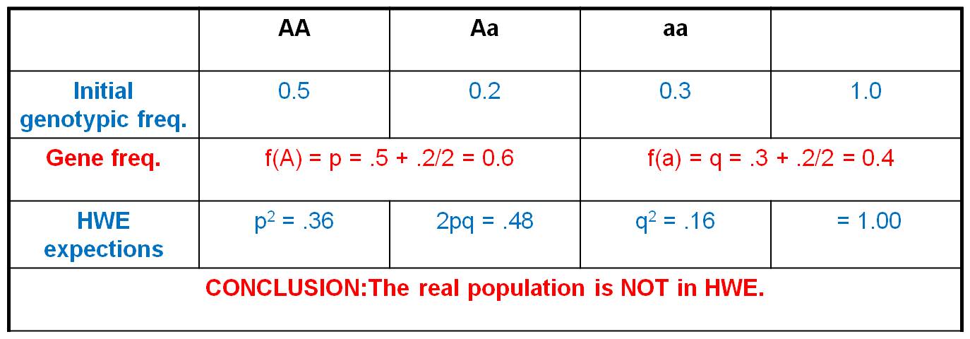
- If no real populations can explicitly meet these assumptions, how can the model be useful?  For instance, no real population is infinitely large, so how can the model be useful?  We use it for COMPARISON.  This model describes what the genotypic frequencies should be IF the population was in equilibrium.  If the real genotypic frequencies are not close to these expectations, then the population is not in HWE.... it is evolving. And if a population is not in HWE, then the population must be violating one of the assumptions of the HWE model.  Think about that.  The HWE is only 'true' if all the assumptions are being met.  If your real population differs from the model, then one of the assumptions must not apply to your real population.  This narrows your focus on WHY the real populations isn't behaving randomly... and it might identify WHY the population is evolving.... which is a biologically interesting question.                

- Again, the coin analogy applies.  No REAL coin is probably exactly perfectly balanced. But, if I give you a coin and ask you how balanced it is, you flip it a few times and compare its behavior to WHAT YOU WOULD EXPECT FROM A PERFECT COIN (50:50 RATIO). Even though a perfectly balanced coin may not exist, we can use this theoretical model as a benchmark, to compare the behavior of real coins.  Many real coins act in a manner that is consistent enough with the expectations from a perfectly balanced coin that we are willing to use them AS IF they were perfectly balanced.   The Hardy Weinberg Equilibrium Model is the same... it is a theoretical model of no change against which we can measure real populations. 

If HWE can be assumed, then the frequency of recessive diseases can be assumed to equal q², and the frequency of carriers in the population can be estimated like this:

1) The frequency of hemachromatosis worldwide is 1/450. If we assume that hemochromatosis is caused by a recessive gene (q), and if we assume the population is in HWE with respect to this trait, then q² = 1/450 = 0.002. So, we take the square-root of both sides to find q = 0.047. Well, if q = 0.047, and if p + q = 1, then p = 1 - 0.047 = 0.953.

2) If q = 0.047 and p = 0.953, then the frequency of heterozygous carriers = 2pq = 0.09. So, we estimate that 9% of the population are carriers.

Now, you might say, "but we just determined that HWE would be unusual; so why would we assume it is true for a given gene?" Well, a deleterious gene has already been largely weeded out of a population, so selection against the few alleles that are left is really weak. Indeed, this condition may not influence reproductive success, anyway (NO SELECTION). In addition, we don't select mates based on whether they have hemochromatosis (I bet you NEVER asked your date if they have hemochromatosis, for example!!), so we can assume there is RANDOM MATING in the population with respect to this trait. And although the human population is not infinite, it is really big (~7 BILLION), so the effect of sampling error is probably very small. Mutation is very rare, so the effects of mutation are likely to be very small. And if we are making an estimate based on the whole human population, then there can be no 'migrants' coming in from somewhere else (Martians?). So, in some cases, we can reasonably assume a population might be in HWE for a given gene. Of course, we could be wrong... and we would test that prediction by sampling individuals in the population and determining the frequency of heterozygotes genetically. But at least we would have a working hypothesis.

  Study Questions:

1.  What are the five assumptions of the Hardy-Weinberg Equilibrium Model?

2.  Consider the following population:

• - calculate the genotypic frequencies.
• - calculate the gene frequencies
• - calculate the HARDY WEINBERG EQUILIBRIUM frequencies.

3. If the HWE model does not describe any real population, how can it be useful?