 Suppose
we do the following dihybrid cross:
Suppose
we do the following dihybrid cross:
Sex linkage showed us that traits can be inherited in a related manner, not just independently. In sex linkage, the transmission and expression of a trait correlated with the transmission of sex chromosomes, so there was a relationship between expressing that trait and expressing a particular sex. Curiously, for x-linked human traits, the relationship is indirect. The gene that causes maleness (sry) is on the Y, but most sex-linked genes are on the X; so the correlation with sex is due to the combination of sex chromosomes received, not due to the inheritance of a single chromosome that governs BOTH these traits.
The pattern with which pairs (or sets) of genes are inherited can actually be much more direct. For example, suppose we consider the pattern of heredity for traits governed by genes on the same chromosome? Then obviously, their pattern of heredity will be directly related. It is this scenario that we examine in this lecture - the pattern of heredity of genes that are linked together as part of the same chromosome.
A critical aspect of this lecture will be understanding the process of crossing-over. As you recall, as the chromosomes condense in Prophase I of meiosis, they condense with their homolog. During this condensation period, homologs can exchange pieces of chromosome. This is called crossing over. Now, because these are homologous chromosomes that have the same loci, an equal exchange means that both chromosomes still have a gene for every trait they govern. However, because the pieces they exchange may contain different alleles for these genes, crossing over can produce new combinations of alleles along the length of each chromosome that did not exist before. You'll see how this works as we go along.
There are some assumptions that we will make here about crossing over:
1) Crossing over is a random event. Where a cross-over occurs along a chromosome is random. (Geneticists have found that this is not explicitly true - there are places where crossing over is more likely to occur...but we will make this assumption here.)
2) So, the greater the DISTANCE between genes on a chromosome, the more likely it is that a random cross-over event will occur between them. Likewise, the probability of a cross-over event declines as the distance between genes declines.
3) So, for genes in a local region of a chromosome, crossing over will be a rare event.
4) And, given this relationship, it means that we can use the frequency of crossing over, if we can measure it, as an index of the distance between the genes. YOU NEED TO UNDERSTAND THIS LOGIC BEFORE GOING ANY FURTHER.
Let's start with the most extreme (and simplest) example. Consider two loci, A and B, that are immediate neighbors on a chromosome; so close that they are always inherited together because the chance that a random cross-over event splits them exactly is ridiculously small.
Suppose
we do the following dihybrid cross:
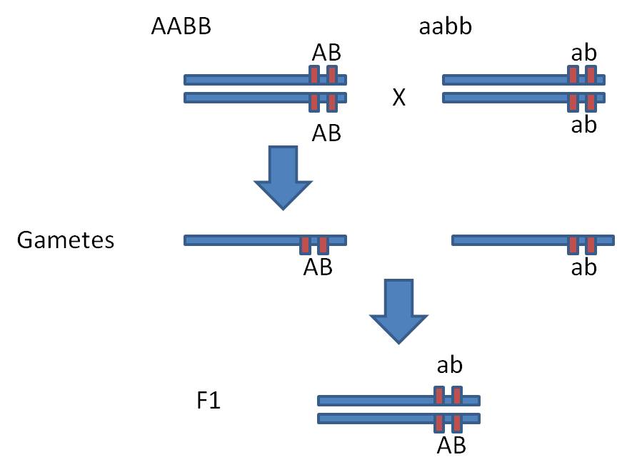
Dihybrid Cross: AABB x aabb = 100% AaBb.
Hmmm... well, so far the results are indistinguishable from independently assorting genes.
 But
now do the F1 x F1 cross. Each parent can only produce two types of gametes,
because the AB genes and the ab genes are parts of the same chromosomes and
do not assort independently. In this case, wherever the "A" goes,
the "B" has to go, too; they are part of the same unit. GIVEN THIS
spatial relationship (with AB linked and ab linked) and no crossing over, each
parent can only produce AB and ab gametes types (and not the additional Ab and
aB types we would expect from an AaBb parent with independent assortment).
[*Of course, the other spatial arrangment
is possible, with the Ab linked together and the aB linked together. But we
would have had to start with different pure-breeding stocks in the parental
generation (AAbb, aaBB). And, if this was the arrangment, then the F1 would
only be able to produce Ab and aB gametes. OK, back to the problem we have!]
But
now do the F1 x F1 cross. Each parent can only produce two types of gametes,
because the AB genes and the ab genes are parts of the same chromosomes and
do not assort independently. In this case, wherever the "A" goes,
the "B" has to go, too; they are part of the same unit. GIVEN THIS
spatial relationship (with AB linked and ab linked) and no crossing over, each
parent can only produce AB and ab gametes types (and not the additional Ab and
aB types we would expect from an AaBb parent with independent assortment).
[*Of course, the other spatial arrangment
is possible, with the Ab linked together and the aB linked together. But we
would have had to start with different pure-breeding stocks in the parental
generation (AAbb, aaBB). And, if this was the arrangment, then the F1 would
only be able to produce Ab and aB gametes. OK, back to the problem we have!]
So, in the F1 x F1 cross, these two genes are inherited as if they were one gene; yielding a 3:1 ratio of AB:ab offspring.
The critical test, of course, is to see what type of gametes this F1 individual can make. And to determine what type of gametes an individual can make, what type of cross do we conduct? Correct, a test cross. In this case, the Test Cross would be: AaBb x aabb. If AB and ab are completely linked, as above, then the progeny would be = 50%AB (AaBb) and 50% ab (aabb); with no Ab or aB offspring because this F1 individual would not make those gamete types.
OK, hopefully you have the idea. Now let's consider the case where we are studying a pair of genes that are in the same region of a chromosome, so that some (rare) crossing over will occur between them. Our goals are:
1) Determine if the genes are linked, or are assorting independently.
2) If they are linked, detemine the arrangement of alleles in the F1 individual; which alleles are paired on each homolog?
3) Determine the distance between loci.
1. Determining if the genes are linked, or are assorting independently:
To do this, we will conduct a Test Cross, so that we can "see" the types of gametes that our F1 individual makes. Then, we can compare these frequencies with expectations derived from the product rule for independent events.
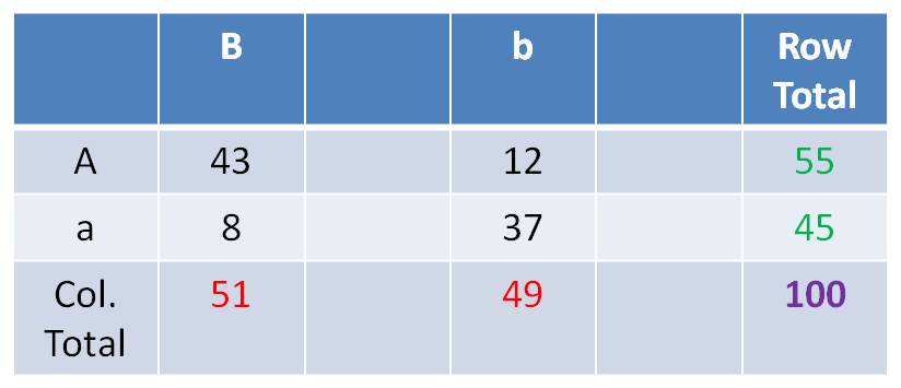
Suppose you did your Dihybrid test cross and got: 43 AB,12 Ab, 8 aB, 37ab
Could these genes be assorting independently? Well, anything is possible, but ARE THESE RESULTS LIKELY from independently assorting genes? How likely? Let's conduct a Chi-Square test of Independence to determine the likelihood of observing these results from independent events.
Determine what you would expect
if the genes assorted independently:
- For the A trait, by itself, there are 55/100 A and 45/100 a.
- For the B trait, by itself, there are 51/100 B and 49/100 b.
- So, if the genes assort independently, you can predict the probability of
phenotypic combinations by multiplying the independent probabilities together.
- Now, multiplying fractions
gives you a fraction. To find the number/frequency of individuals, you have
to multiply this final fraction times the sample size (100 in this case). So,
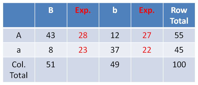
your expected frequencies, under the hypothesis of independent assortment, are:
 The
frequency of ‘AB’ should = f(A) x f(B) x N = 55/100 x 51/100 x 100
= 28
The
frequency of ‘AB’ should = f(A) x f(B) x N = 55/100 x 51/100 x 100
= 28
The frequency of ‘Ab’ should = f(A) x f(b) x N = 55/100 x 49/100
x 100 = 27
The frequency of ‘aB’ should = f(a) x f(B) x N = 45/100 x 51/100
x 100 = 23
The frequency of ‘ab’ should = f(a) x f(b) x N = 45/100 x 49/100
x 100 = 22
You can calculate these in a 2 x
2 Chi-square Test of Independence Table as:
(Row Total x Column Total)/ Grand Total.
So, the expected frequency of AB individuals = (51 x 55)/100 = 28
 Compare
observed vs. expected using the chi-square computation: X2 = SUM
[(o-e)2/e]:
Compare
observed vs. expected using the chi-square computation: X2 = SUM
[(o-e)2/e]:
| Obs. | Exp. | (o-e) | (o-e)2/e | |
| AB | 43 | 28 | 15 | 8.04 |
| Ab | 12 | 27 | -15 | 8.33 |
| aB | 8 | 23 | -15 | 9.78 |
| ab | 37 | 22 | 15 | 10.23 |
| Sum = | 36.38 |
- Interpreting the Chi-Square Value of 36.38 - Statisticians have determined how likely particular chi-square values are, just by chance, if the events truly ARE independent. They have determined that, with 1 'degree of freedom' (what you have: (rows - 1)(columns - 1) )), independently occurring events will only produce a score of 3.84 only 5% of the time. A score of 6.63 will only occur 1% of the time, just by chance, when two events truly ARE independent. Larger scores are progressively less likely, because greater deviations from the expectations are less probable (for events that ARE independent). Your score of 36.38 signifies that truly Independently Assorting genes would ONLY yield results this deviant from what you would expect less than 1% of the time. - So, independently assorting genes are unlikely to yield your results. There is less than 1 chance in 100 that independently assorting genes would produce results that deviate this much from expectations. Can I say it any other way?
- So, the most appropriate conclusion is to reject the hypothesis of independence, and conclude that your genes are NOT assorting independently. You should conclude that they are linked.
HAVING CONCLUDED THAT THE GENES ARE LINKED, WE CAN NOW ANSWER TWO OTHER QUESTIONS.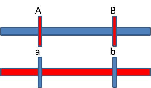 2)
Detemining the arrangement of alleles in the F1 individual; which alleles are
paired on each homolog?
2)
Detemining the arrangement of alleles in the F1 individual; which alleles are
paired on each homolog?
If crossing over is rare, then most of the time it does NOT occur. So, most of the time, the alleles are passed to the offspring in their original arrangement in the F1 individual - and these phenotypes should be the most abundant phenotypes in the offspring. In our case, these are the AB and ab phenotypes. So, the original AaBb parent had the A and B alleles on one chromosome and the a and b alleles on the other homologous chromosome. MOST OF THE TIME, the allelic combinations were inherited as a unit. These gametes are called the "parental types", because the preserve the original spatial combination of alleles that existed in the parent.
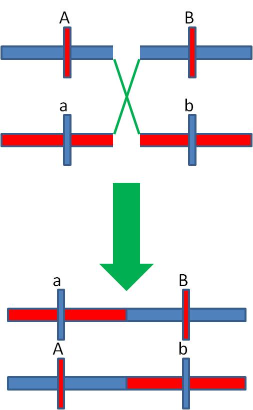 When
a rare cross-over occurs between these loci, the Ab and aB gamete types are
produced. These are less common than the parental types (becasue crossing over
is rare), and they are called the "recombinant types".
When
a rare cross-over occurs between these loci, the Ab and aB gamete types are
produced. These are less common than the parental types (becasue crossing over
is rare), and they are called the "recombinant types".
3. Determining the distance between loci:
Well, now we apply another assumption: that the frequency of crossing over is proportional to the distance between loci. So, we measure the frequency of crossing over and can use that as a direct index of the distance between loci. So, there were 12 Ab and 8 aB offspring... for a total of 20 offspring produced by recombination events. This is 20.0% (20/100 offspring). So, we say that the genes are 20.0 map units (or centiMorgans) apart. Genes that are closer together will recombine less often... genes that are farther apart will recombine more often.
 D.
Summary
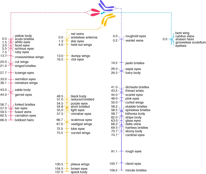
D.
SummarySo, by observing the frequency with which pairs of traits are inherited, we can build maps of the physical location of genes on chromosomes. The pioneers of this method were T. H. Morgan, who first described sex linkage in the early 1910's, and his student A. Sturtevant, who conducted many breeding experiments with Drosophila and began construction of what is known as a linkage map. The one shown here is a partial linkage map for Drosophila - constructed through heredity experiments using fruit flies. Linkage maps are very important, and they remain important today, even though we now have other ways to map DNA - like by the sequence of A, C, T, and G. However, sequence maps don't show us the spatial relationship of genes that govern particular traits. In order to know which sequence might code for a given trait, we need to compare the known location for a sequence with the known location of a gene governing a trait from a linkage map. This can actually be very difficult, because the scales of resolution are so different. Through construction of a linkage map, we might estimate that a trait is governed by a gene that is 5 centiMorgans from the centromere of the chromosome. But each centiMorgan covers thousands of base pairs, and the map location of this gene covers thousands of base pairs, too. Finding the particular sequence within this region still requires additional work. So, mapping through linkage analysis is still very important, and we are still finding the locations of human genes based on the frequency with which they are inherited with known genes, or known DNA sequences called 'markers'.
Study Question:
Consider these results from the following testcross:
AaBb x aabb
F1 Phenotypes:
AB 15
Ab 22
aB 29
ab 13
Conduct a chi-square test of independence. Using the p = 0.05 level (and critical X2 of 3.64), make a conclusion about whether the genes are linked or assort independently.
If the genes are linked, map their positions in the heterozygous parent, showing which alleles are on which homolog, and determining the distance between loci.