 3.
Non-Random Mating:
3.
Non-Random Mating:
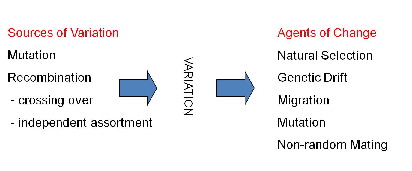
As we've seen, equilibrium can only occur if ALL of the assumptions are met. If they are not met, then the population will evolve. We are now going to look at each assumption, and consider what happens when each assumption is violated. This will show us how evolution can occur by each of these different agents of evolutionary change.
1. Mutation
Although large scale mutations like polyploidy can cause instantaneous speciation, what we are talking about here are substitution mutations that change one allele into another, or make a new allele. Although such changes are very important sources of new variation, they do not change the genetic structure of a population very much at all, even when they occur: these mutations are rare, usually occurring at a rate of 1 x 10⁻⁴ to 1 x 10⁻⁶.
Consider a population with:
f(A) = p = 0.6
f(a) = q = 0.4
Suppose 'a' mutates to 'A'
at a realistic rate of: µ = 1 x 10⁻⁵ . How will this rate of
mutation change gene frequencies? Not much: 'a' will decline by: qm = .4 x 0.00001
= 0.000004
'A' will increase by the same amount. So, the new gene frequencies will be:
p1 = p + µq = .600004, and q1 = q - µq = q(1-µ) = .399996.
So, mutation is a very important source of new alleles, but it doesn't change
the gene frequencies in a population very much.
2. Migration
Consider a resident population in which p = 0.6 and q = 0.4. Suppose immigrants migrate into this population, bringing A and a alleles into the population at these frequencies: p =0.8 and q = 0.2. The effect of this influx will depend on the number of immigrants relative to the number of residents. 100 immigrants may not change the genetic structure of a population containing 1 million residents, but they could have a dramatic effect on a population of 100 residents. We measure this relative effect by quantifying the proportion of the total combined population that are immigrants. So, in our example, suppose so many immigrants move in that they represent 10% of the new, combined population. We calculate new p as a weighted average based on fraction of immigrants and residents:
So, p1 = (0.6)(0.9) + (0.8)(0.1)
= 0.54 + 0.08 = 0.62
residents contribute p at a rate of 0.6, and they represent 90% of the combined
population. Immigrants contribute p at a rate of 0.8, and they are 10%
of the population.
q1 = (0.4)(0.9) + (0.2)(0.1)
= 0.36 + 0.02 = 0.38, so we have done our math right because 0.62 + 0.38 = 1.0
There are two possible evolutionary effects. First, migration will make two populations similar to one another; particularly if the rate of immigration is high or the process is continuous over time. Migration can also introduce new alleles into a population, but again this effect will be correlated with the abundance of immigrants relative to the number of residents.
3.
Non-Random Mating:
a. Positive Assortative Mating
There are many ways that non-random mating can occur. We will look at a couple. The first example is called "positive assortative mating". This is where mates 'sort' themselves with others of the same genotype. This can be thought of as "like mates with like". So, consider our old four o'clock plants with incomplete dominance. A population might contain red, pink, and white flowers. Suppose the red flowers open in morning, and are pollinated just by hummingbirds (that prefer red flowers). Suppose the white flowers open at night, and are pollinated by moths. And suppose the pink flowers open in the afternoon, and are pollinated by bees and butterflies. In this case, "like mates with like" for flower color (and time of opening). So, a plant with red flowers will only mate with another plant having the same genotype for (red) flower color. Now, it is IMPORTANT to realize that plants are only positively assorting for flower color and opening time in this case. One red flowering plant may be tall while the other is short; one may have hairy leaves while the other has smooth leaves. Indeed, the plants may be mating at random with respect to all other traits.
When AA individuals mate only with each other, all their offspring will be AA, as well. So, if 20% of the population is AA (intial genotypic frequency = 0.2), and if there is no difference in reproductive success (because we are only violating the assumption of random mating so there is no selection), then these parents will make 20% of the offspring and they will all be AA. The same goes for aa individuals only mating with other aa individuals - all their offspring are aa. However, when Aa heterozygotes only mate with one another, they produce AA, Aa, and aa offspring in a 1/4:1/2:1/4 ratio. If 60% of the population is heterozygous, then they will make 60% of the offspring... but these offspring won't all be heterozygous; only 1/2 - or 30% will be heterozygous. 15% will be AA and 15% will be aa. So, the total frequency of AA offspring in the F1 will be 35%; 20% had AA parents and 15% had Aa parents.
As a consequence of positive assortative mating, the frequency of heterozygotes will decline and the frequency of homozygotes will increase. Curiously, the gene frequencies won't change, so in the F1, f(A) = .35 + 0.30/2 = 0.5... just as it was in the orginal population (f(A) = 0.2 + 0.6/2 = 0.5). The genes are just being 'dealt' to offspring in a non-random manner, affecting the genotypic frequencies at this locus.
So, suppose we observed the F1 population in nature, and wanted to know if it was in HWE. We would calculate the gene frequencies (A = 0.5, a = 0.5), and then estimate what the frequencies of the genotypes would be IF the population was in HWE: p2 = 0.25, 2pq = 0.5, q2 = 0.25. We would compare our real population's genotypic array with this HWE expectation, and see that they are not the same. And we could see one thing more... we would see that the ACTUAL OBSERVED frequency of heterozygotes (0.30) is LESS THAN the expected frequency of heterozygotes under the HWE hypothesis (0.5). And we would see that the observed frequency of both homozygotes is greater than expected. Knowing that positive assortative mating can cause this pattern, we would have a working hypothesis regarding the agent of evolution at work in this population.
b. Inbreeding: Mating with a Relative
Inbreeding is mating with a relative. It is similar to positive assortative mating, except that the two mates are not just similar at one locus, but they are probably similar at MANY loci because they are related and got their genes from the same ancestors. Siblings share, on average, half their genes. Matings between siblings, then, will tend to reduce heterozygosity at MANY loci, not just one.
The most extreme example is "obligate self-fertilization". This is where a hermaphrodite ONLY mates with themselves. This is not asexual reproduction - they produce gametes by meiosis and get all the benefits of producing variable gametes that occurs in sexual reproduction; but they only fertilize their own gametes. This has a profound effect on the genetic structure of the population. Think about it: when an organism mates with themselves, they are mating with an organism that has the SAME genotype at EVERY locus. So, there will be a decrease in heterozygosity across the entire genome, with a 50% reduction in heterozygosity each generation. This is the most rapid loss possible. Siblings are only related, on average, by 50%, so the loss of heterozygosity will only occur 1/2 as fast.... but it will still occur at all loci across the genome.
Inbreeding often reduces reproductive
success, because there is an increase in homozygosity - and this means that
deleterious recessives are going to be expressed more frequently and exert their
negative effects on the offspring. A deleterious allele may be rare in a population,
but inbreeding will increase the probability that it occurs in the homozygous
condition and is expressed. Because inbreeding can reduce the survivorship of
offspring and thus reduce reproductive success of the parent, it is often selected
against. Selection favors different strategies that reduce the likelihood of
inbreeding, like "self-incompatibility" in some plants, like lions who push
male cubs out of a pride when they mature (thus they don't breed with their
sisters), or like humans who have a variety of cultural taboos against breeding
with relatives. However, inbreeding is also a mechanism for purging deleterious
alleles from the population. If a population can get through the first
few generations in which homozygote recessive are produced and selected against,
the net effect will be to eliminate these deleterious alleles from the population.
That can be a good thing in the long run.
4. Populations of Finite Size and Sampling Error/"Genetic
Drift"
The genetic structure of a population can change from generation to generation
just by chance - through a process statisticians call "sampling error"
and geneticists call "genetic drift". Think about it this way: suppose
we have a very large population in which p = 0.3 and q = 0.7, and the population
is in HWE to start; so the f(AA) = 0.09, f(Aa) = 0.21, and f(aa) = 0.49. Now,
suppose only 4 individuals mate, and suppose those four are just 'lucky' - they
don't mate because they are better adapted in any way, they just got lucky.
It is very unlikely that these four individuals will have the same genetic structure
as the whole population; small samples are notoriously unrepresentative and
variable. Indeed, all four may be 'aa', and the population will have changed
dramatically, losing the 'A' allele. This is why, to have confidence in any
observed pattern, you want a large sample. So, a population's genetic structure
may change just due to chance.
There are two important patterns that result from this effect:
First, small samples will tend to differ more from the original population than large samples. Second, since the direction of this change is random, multiple small samples will tend to vary more from one another, on average, than multiple large samples. So, small populations will diverge more rapidly from one another, due to drift, than large populations.
There are two biological situations where these effects are particularly important. The first is called a "Founder Effect", where a small number of colonists establish a new population that is isolated from the original population. Because this population of "founders" is small, it is likely to differ dramatically from the original population.... and because it is small, it will also chance quickly just due to drift, as the simulations in lab showed.
The second important instance in which drift is important is called the "bottleneck effect". This is when a large population is reduced in size. Typically this reduction is caused by predation, a pathogen, or an environmental change. The survivors usually make it because of selection at certain loci. For instance, survivors of a pathogenic infection may be resistant to the pathogen. However, at other loci, the reduction in population size causes genetic change due to drift.
So, CHANCE can be an agent of evolutionary change. CHANCE, especially in small populations, can cause changes in the genetic structure of a population. This is NOT selection - selection is "non-random reproductive success" - the organisms that breed are "better" than the others. Here, in Genetic Drift, the breeders are just LUCKY, not better. It is random change. And, as the computer modes demonstrate, populations will tend to become different genetically 'simply by chance', because these chance changes are unlikely to be the SAME changes, or in the same direction, from population to population. So, we can't STOP populations from evolving, really - they will all change over time, even just do to random sampling error, and they will tend to become different from other populations of the same species. Of course, if the populations are very large, these random patterns of divergence will be very slow.... but since no population is infintie in size, these random changes will necessarily occur over time.
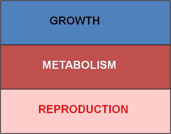
5. Natural Selection
1. Fitness Components:
As you know, natural selection is
"differential reproductive success" in a genetically variable population.
We can measure lifetime reproductive success as the number of successfully reproductive
offspring that a genotype produces, on average. This measureable quantity is called
"fitness". There are three factors that can influence 'fitness', or
reproductive success:
Now, it seems like natural selection would favor organisms that maximized all three components; and it would if that were possible. However, organisms can't maximize all three components because there are energetic constraints - organisms only have so much energy in their 'energy budget'. So, maximizing one component results in less energy that can be invested in the other two. In addition, there are contradictory selective pressures in the environment, such that a characteristic may increase fitness with respect to one variable but decrease it with respect to another variable. These are called 'trade-offs', and we will now examine these in more detail.
2. Constraints:
 a.
finite energy budgets and necessary trade-offs:
a.
finite energy budgets and necessary trade-offs:
The most obvious constraint is ENERGY.
Every organism has a finite energy budget; it has harvested only so much energy
from the environment that it can allocate to all of its activities. There
are three major expenses:
So, with limited energy, increasing one thing means that you must reduce costs in another area. These patterns of energy allocation have direct effects on different fitness components.
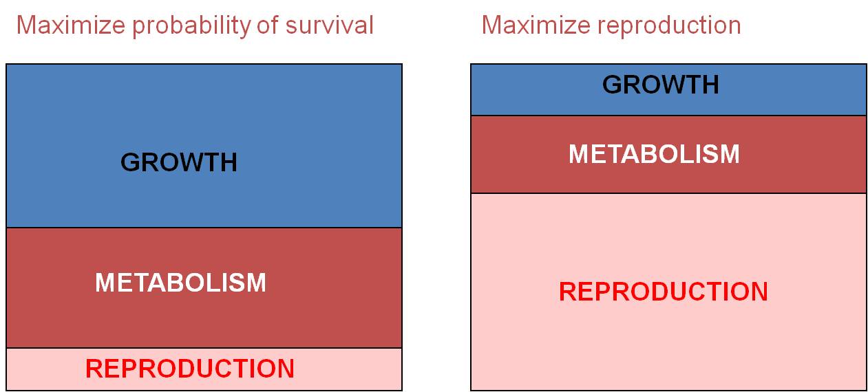 Trade-Off
#1: Survival vs. Immediate Reproduction: For example, ff an organism
maximizes energy investment in growth and metabolism, then they will increase
the probability that they survive. Why? Because being large tends to increase
the probability of survival, if only because there are fewer things that can
eat you. Likewise, large organisms are not as sensitive to changes in the environment.
Simply because of their larger size (and smaller surface area/volume ratio),
they don't lose heat, salt, water, or other materials to the environment as
rapidly as small organisms. However, by investing in growth, this means that
there is LESS energy to invest in immediate reproduction, meaning fewer offspring
can be produced. So, you CAN'T maximize all three components of selection
at the same time; selection seeks the best compromise in a given environment,
with particular biological potentials and constraints. Many organisms invest
in growth when young, to develop as rapidly as possible through these early,
vulnerable life-history stages. They delay reproduction completely when
they are young to maximize growth rate. Then, after they are older and
larger, they invest energy in reproduction (and growth rate SLOWS). These
organisms are "perennial" or "K" strategists - they are long-lived
organisms. Other organisms take a different strategy. They reproduce
early at the expense of growth. They don't survive long as a consequence
- they are "annual" or "r" strategists - species that live for less
than a year but invest almost all their energy in immediate reproduction. These
two examples are opposite sides of the same coin - they are both examples of
this same trade-off between survival and immediate reproduction; organism can't
maximize both at the same time, so they tend to maximize one or the other, or
change their pattern of allocation through their life.
Trade-Off
#1: Survival vs. Immediate Reproduction: For example, ff an organism
maximizes energy investment in growth and metabolism, then they will increase
the probability that they survive. Why? Because being large tends to increase
the probability of survival, if only because there are fewer things that can
eat you. Likewise, large organisms are not as sensitive to changes in the environment.
Simply because of their larger size (and smaller surface area/volume ratio),
they don't lose heat, salt, water, or other materials to the environment as
rapidly as small organisms. However, by investing in growth, this means that
there is LESS energy to invest in immediate reproduction, meaning fewer offspring
can be produced. So, you CAN'T maximize all three components of selection
at the same time; selection seeks the best compromise in a given environment,
with particular biological potentials and constraints. Many organisms invest
in growth when young, to develop as rapidly as possible through these early,
vulnerable life-history stages. They delay reproduction completely when
they are young to maximize growth rate. Then, after they are older and
larger, they invest energy in reproduction (and growth rate SLOWS). These
organisms are "perennial" or "K" strategists - they are long-lived
organisms. Other organisms take a different strategy. They reproduce
early at the expense of growth. They don't survive long as a consequence
- they are "annual" or "r" strategists - species that live for less
than a year but invest almost all their energy in immediate reproduction. These
two examples are opposite sides of the same coin - they are both examples of
this same trade-off between survival and immediate reproduction; organism can't
maximize both at the same time, so they tend to maximize one or the other, or
change their pattern of allocation through their life.
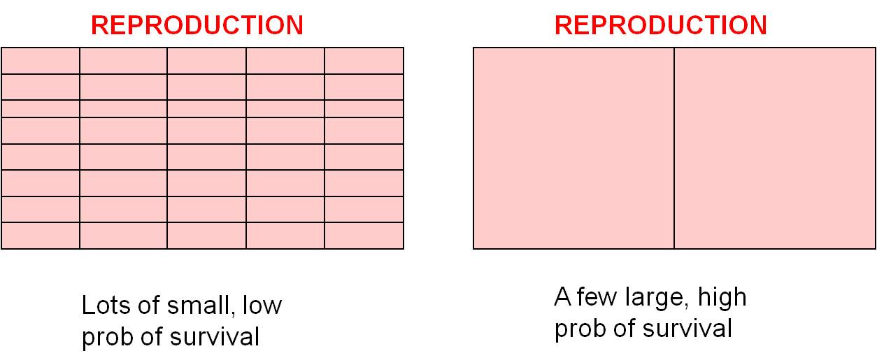 Trade
Off #2: Offspring Number vs. Offspring Size/Survivorship: There are
also trade-offs within the reproduction budget (the pink section in the budgets,
above). For the same "energetic cost", you can make lots of little offspring
or a few big offspring. As we discussed above, small organisms have a lower
probability of survival than large organisms, so you can make lots of small
offspring that each have a small chance of surviving, or you can invest in fewer
offspring and increase their chance of survival (by making them larger or by
investments in parent care). Small organisms, like insects, can't really make
a big offspring, so they exploit the other strategy and make lots of small offspring.
Large organisms can really take advantage of this 'choice', and selection will
favor different strategies in different large organisms. Some organisms
like mammals and birds tend to produce a few large offspring and invest significant
amounts of energy in parental care, further increasing the probability that
the offspring survive. Large vertebrates without parental care, like many
reptiles, produce more numerous smaller offspring and 'play the lottery' - increasing
the chance that one offspring survives by producing more offspring.
Trade
Off #2: Offspring Number vs. Offspring Size/Survivorship: There are
also trade-offs within the reproduction budget (the pink section in the budgets,
above). For the same "energetic cost", you can make lots of little offspring
or a few big offspring. As we discussed above, small organisms have a lower
probability of survival than large organisms, so you can make lots of small
offspring that each have a small chance of surviving, or you can invest in fewer
offspring and increase their chance of survival (by making them larger or by
investments in parent care). Small organisms, like insects, can't really make
a big offspring, so they exploit the other strategy and make lots of small offspring.
Large organisms can really take advantage of this 'choice', and selection will
favor different strategies in different large organisms. Some organisms
like mammals and birds tend to produce a few large offspring and invest significant
amounts of energy in parental care, further increasing the probability that
the offspring survive. Large vertebrates without parental care, like many
reptiles, produce more numerous smaller offspring and 'play the lottery' - increasing
the chance that one offspring survives by producing more offspring.
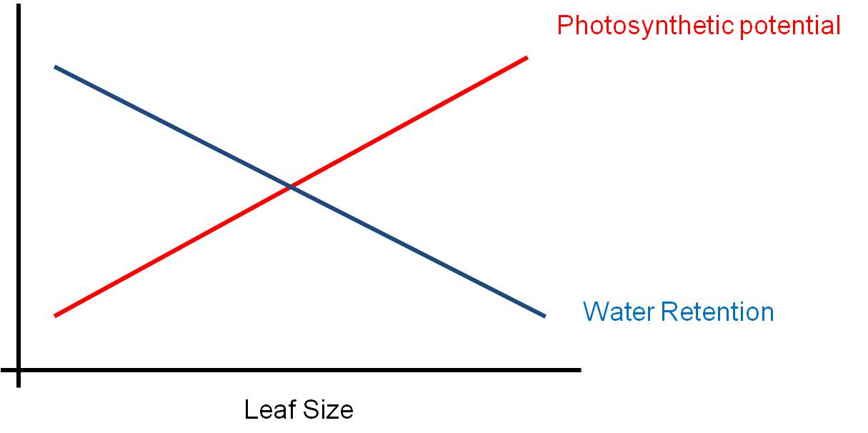
b. Contradictory environmental pressures:
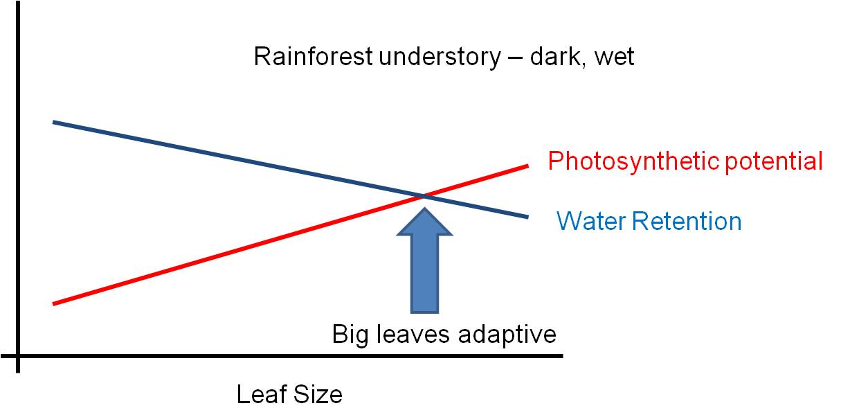
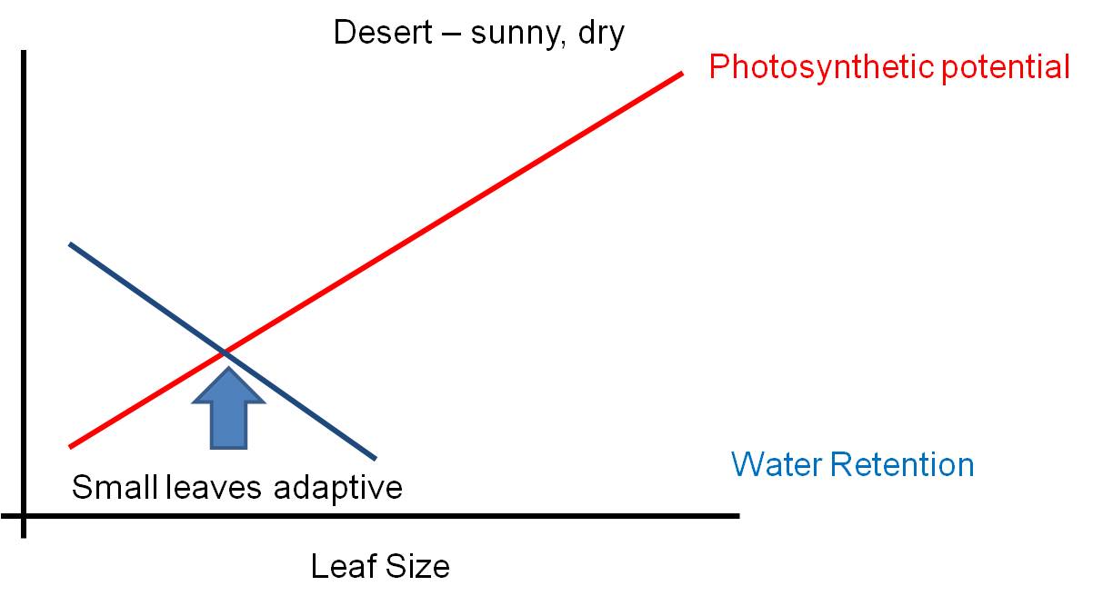
The environment is a complex place - there are pressures that might favor some structures, and other pressures acting AT THE SAME TIME that might select against that trait. Selection can not maximize BOTH responses at the same time - so the solution will be a suboptimal compromise. Consider leaf size. Big leaves are GOOD for light absorption - they represent a larger solar panel that intercepts more light. But big leaves are BAD for water loss - with a large SA/V ratio, water is lost rapidly from a large thin leaf. So, the size of a leaf will be a compromise solution to these two pressures... a solution that maximizes neither function. The 'adaptive compromise' size depends on the relative strengths of the contradictory pressures. If the risk of water loss is low (like in a rainforest), then the leaf can be large. If the risk of water loss is high (like in the desert)and there is strong sun, then the selective pressure to reduce leaf size is strong and leaves will be small or non-existent (cacti).
For these reasons, 'perfect' adaptations are impossible; there are biological costs to any adaptation (in terms of 'opportunity costs' - NOT being able to do something else as well),and in terms of the complex nature of the environment where selective pressures can be contradictory.
 |
 |
 |
3. Modeling Selection:
 a.
Calculating relative fitness:
a.
Calculating relative fitness:
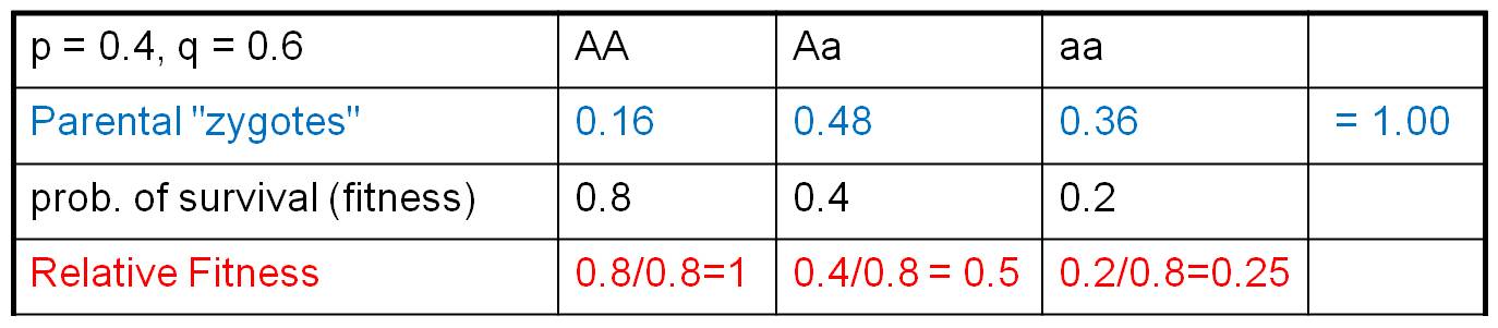
Consider the population to the right. Suppose a population has JUST mated, creating parental zygotes in the genotypic frequencies shown. Let's suppose that these zygotes, as a consequence of their genotypes at this locus, have different probabilities of surviving to reproductive age. But, to make things simple, lets assume that the other two components of fitness are equal across the genotypes. So, differences in FITNESS are only influenced by differences in the probability of survival to reproductive age. Suppose those survival probabilities are 0.8, 0.4, and 0.2, respectively (as shown).
These probabilities of survival are 'absolute' fitness values. Curiously, absolute fitness values are not very informative. What is important is relative reproductive success - reproductive success relative to the other genotypes in the population. Think about it this way... suppose I tell you that "I am thinking of an AA genotype that produces 1000 offspring a year. Do you think the f(A) will increase or decrease in the population as a consequence of selection?" Well, you might think, "wow, 1000 offspring is ALOT! Surely the f(A) will increase!" But this would be an incorrect assumption. You need to know what type of organism I am talking about, and how reproductively successful the other genotypes are in the population. If this organism is a salmon, then 1000 offspring might be more than other genotypes in the population. But if this organism is a clam, then the other genotypes might be producing 10's of thousands of offspring - and the F(A) will decline. So, the key to selection is differential reproductive success, which means reproductive success relative to other organisms in the population. We represent this as RELATIVE FITNESS, and calculate it by dividing all fitness values by the LARGEST (ie., most FIT) value. This means that one genotype will necessarily have a RELATIVE FITNESS = 1. In our case, above, we divide each fitness value by the greatest value (0.8), so the relative fitness values are "1, 0.5, and 0.25" for AA, Aa, and aa genotypes, respectively.
 b.
Modeling Selection:
b.
Modeling Selection:
Now let's see what effect this selection
(in terms of differential survival) has on the genetic structure of the population.
First, we multiply the initial genotypic array by the relative fitness values.
For us, this describes the relative proportion of zygotes surviving to reproductive
age. So, these are the same organisms - we don't have a new generation yet -
it is just that the original zygotes have grown up and survived to adulthood
at different rates. Since many organisms have died, these genotypic values no
longer sum to 1. They sum to 0.49. If we want to know what the genotypic frequencies
are in the population of surviving reproductive adults (and WE DO), then we
must know what part of this new total is represented by each genotype. We calculate
that by dividing each genotypic value by the total (0.49), producing the genotypic
frequencies in this breeding population. These, of course, now sum to 1. From
here, we are home free. we calculate the gene frequencies in this reproductive
gene pool as:
F(A) = f(AA) = f(Aa)/2 = 0.575, and
f(a) = f(aa) + f(Aa)/2 = 0.425.
These sum to 1 so we've done the math correctly. Now, to produce the F1 zygotes,
assume that all other conditions of HWE are met (we are only modelling the direct
effect of selection, alone), so we assume that the organisms mate randomly and
calculate the genotypic frequencies of zygotes in the F1 using the terms: p2,
2pq, and q2.
So, as the result of differential survival to reproductive age, A's and a's have not been transferred at the same rate. The intial frequency of these genes was f(A) = 0.4 and f(a) = 0.6. After one generation of differential reproductive success, the gene frequencies have changed dramatically; now the 'A' gene is more abundant.
The period from 1900-1940 was a very exciting and dynamic period in biology. With the rediscovery of Mendel's principles, it seemed that biology had become a truly mathematical, predictive science. The ability to predict patterns of heredity, and the transmission of 'mutant' genes through generations, had a profound impact on evolutionary biology, too. Many geneticists came to view mutation as the primary agent of evolutionary change - not just as a primary source of variation. They viewed Darwin's ideas of probabilistic Natural Selection as too weak to be responsible for the changes seen in the fossil record. However, supporters of Darwin like Ernst Mayr argued that random mutation could not explain the non-random adaptations that were so obvious and pervasive in the natural world. The models of Hardy and Weinberg, in the hands of new population geneticists like Theodosius Dobzhansky and Sewall Wright, were pivotal in resolving this dilemma. The resolution came in the Modern Synthetic Theory of Evolution, developed by these scientists and others in the 1930's and 1940's. As a consequence of the models you have just seen, biologists realized that mutations were too rare to explain the changes seen in natural populations over time. Rather, although mutation and recombination were important as a source of new genetic variation, natural selection and genetic drift were the primary agents that caused the genetic structure of population to change over time. And so, as of 1940, our model of evolution looked like this:
One of the most remarkable things about multicellular life is the co-ordinated activity of cells. Think about it - you are sitting here "reading" - which is to say that light is impinging on cone and rod cells in your retina, electric impulses are created in these cells and passed to intermediary cells and to your optic nerve, and finally to the nerve cell bodies in the visual cortex in your brain. Here, through processes yet to be described, the emergent property of conscious thought makes sense of the pattern of excitation among these neurons and you interpret the perception of these black squiggles to mean something conceptually; a concept that you have encoded as a memory - probably as a particular combination of neuron cell firings in another part of your brain. At the same time, there are other electrical feedbacks between cells that are unconsciously adjusting muscle cells that regulate the aperture of your iris and the shape of your lens to maximize focus and visual acuity as you read. Red blood cells in your circulatory system are nourishing your brain with oxygen, propelled by the contraction of heart muscle cells. Glucose is in your blood, too; produced by the action of digestive enzymes secreted by other cells in your digestive tract, stored for a time in your liver, and released to your bloodstream under chemical cues from the cells in your pancreas. And other cells in you arm contract, causing you to unconsciously scratch the hair follicle cells on your head. Each of us - and every other complex multicellular organism - is composed of millions to trillions of cells that act in a co-ordinated way that maintains the lives of all of these cells and the organism they comprise. And whale cells are swimming through the oceans right now, doing whale things... and dragonfly cells are crawling through the mud at the bottom of the pond, doing dragonfly things. It's no wonder that it took about 3 billion years for life to evolve multicellularity - achieving a level of sophisticated communication and co-operation among microscopic and 'unconscious' cells is quite a feat! If this doesn't make you stop to consider how wonderful life is, then maybe biology isn't the right major for you!
Oh, and let's make it even more amazing. All of these cells that do such remarkably different things in your body are all THE SAME genetically. (This is a pretty important point: the differences in cell function DO NOT arise because different cells have different genes. Rather, all cells have ALL your genes, and different cells just read different subsets of genes and make differnt proteins.) You began your existence as a fertilized zygote - the fusion of your father's sperm and your mother's egg. This single cell divided by mitosis to form 2, then 4, then 8, then 16 cells. All these cells were identical, inheriting the complete genome from the zygote through these mitotic divisions. The process continued, with cells dividing by mitosis to produce the trillions of cells that comprise your body. Although somatic mutations occurred along the way, making some cells a little different, by and large all the cells in your body have the SAME genes. Again, these cells differ in shape and function because they read different parts of your genetic recipe book. Brain cells read recipes for neurotransmitters, and stomach cells read recipes for digestive enzymes, but BOTH neurons and stomach cells have genes for neurotransmitters and digestive enzymes. We belabor the point, but it is an essential fact that you must know from now on.
In this lecture, we are going to look at how genes get turned 'on' and 'off' in cells. We will use examples from bacteria and yeast, which are both single celled. However, by the logic presented above, you should see WHY these regulatory pathways, which function in much the same way in multicellular organisms, is so important to the history of life on earth and to your own personal existence.
Regulation reprise: We have already talked about gene regulation. At the end of the lecture on protein synthesis, there was a brief overview of how this process can be regulated. The accessibility of the gene can be regulated by histones, the binding and action of the RNA polymerase can be regulated by transcription factors, the m-RNA can be spliced differently in different cells to produce different products, the initial protein product can be spliced and/or modified differently in different cells to make different products, and environmental factors can influence how these things are done. Here, we are going to take a look at a couple of those processes in a bit more detail.
Some genes are on all the time in every cell - these are called constitutive genes. Can you think of genes that would have to be on in every cell? Well, all organisms need to be making phospholipids all the time, so I bet the genes that code for enzymes invovled in the production of phospholipids are on all the time. Genes for helicase and RNA polymerase, and for ribosomal proteins are probably on all the time in all cells, otherwise protein synthesis for the whole cell would shut down.
Other genes, however, are regulated. In some cases, the presence of another molecule turns the gene 'on' - these are inducible systems and the molecule that turns the gene on is called the inducer. Other molecules may turn a gene 'off' - this is a repressible system and the molecule that supresses gene activity is called a repressor. Inducers and repressors often bind to the DNA directly to exert their effects, usually upstream from the gene.
In E. coli bacteria, some genes that produce proteins involved in the same reaction are turned 'on' as a group - as a functional - or operational - unit. This unit is called an 'operon'. The lac operon is a functional unit of DNA that codes for three different enzymes involved in lactose metabolism - they influence the absoprtion of lactose and the splitting of lactose into glucose and galactose. So, this operon is used when glucose is needed by the cell and lactose is available. Curiously, these genes only get switch 'on' when lactose is present and glucose is absent - the exact environmental conditions under which the production of these genes that metabolize lactose and produce glucose would be adaptive. But how does this little bacterium know? How does it know that lactose is present and glucose is absent, and that it should turn on its genes? Well, it doesn't know. But bacteria that make these metabolic choices are strongly selected for, because the bacteria only make the enzymes when the enzymes are needed. This saves energy; energy that the bacteria can spend on other things like reproduction. (Selection is differential reproductive success...)
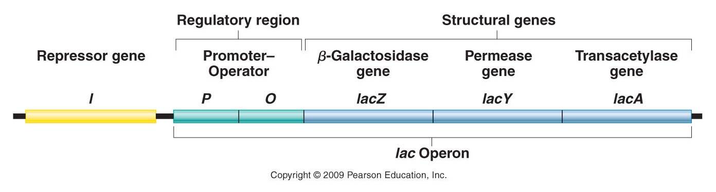 1.
The structure of the operon
1.
The structure of the operon
- The three genes in the lac operon code for b-galactosidase (that cleaves lactose into glucose and galactose), permease (that increases the uptake of glucose), and transacetylase (also required for the process of lactose metabolism).
- Upstream from these genes is the Promoter, where the RNA Polymerase will bind before it transcribes the sense strand in these genes and makes the m-RNA product.
- Between the promoter and the genes is the 'operator' - the region where regulatory elements bind to disrupt or encourage transcription.
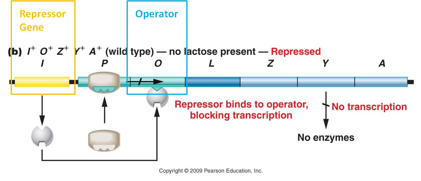
Elsewhere in the genome is the repressor gene, which codes for the repressor protein.
 2.
Induction of the lac operon by lactose
2.
Induction of the lac operon by lactose
Jacob and Monod constructed this operon model of gene regulation in 1960, and they hypothesized that it was an inducible system. The repressor gene produced the repressor protein that, in the absence of lactose, binds to the operator region in the operon. The binding of this protein blocks the RNA polymerase from transcribing the genes, so the genes are 'off'. In the presence of lactose (the inducer), lactose binds to the repressor and changes the repressor's shape. With the new shape, the repressor can no longer bind to the operator and block RNA polymerase. So, RNA polymerase transcribes the genes and the enzymes for lactose metabolism are produced. Eventually the lactose levels decline, the inhibition on the repressor is released, and the repressor can bind again to the operator and stop transcription. So, the enzymes that are used to metabolize lactose are only produced when lactose is present. This is a very adaptive, energetically efficient system.
 Mutant
analyses confirmed the model. A mutation in the operator changed the binding
site for the repressor, and the repressor couldn't bind. so, the genes were
'on' all the time, even in the absence of lactose. Changes to the repressor
gene caused two effects. Changes to the operator binding site meant that it
couldn't bind the operator and couldn't block transcription. Changes to the
lactose binding site meant that it would ALWAYS bind the operator because it
would not bind lactose and change shape.
Mutant
analyses confirmed the model. A mutation in the operator changed the binding
site for the repressor, and the repressor couldn't bind. so, the genes were
'on' all the time, even in the absence of lactose. Changes to the repressor
gene caused two effects. Changes to the operator binding site meant that it
couldn't bind the operator and couldn't block transcription. Changes to the
lactose binding site meant that it would ALWAYS bind the operator because it
would not bind lactose and change shape.
Study Questions:
1. Consider a population with p = 0.8 and q = 0.2. If the mutation rate of A--> a = 4.0 x 10⁻⁶, what will the new gene frequencies be in the next generation?
2. Consider a population, p = 0.8 and q = 0.2. If migrants enter this population with p = 0.1 and q = 0.9, such that immigrants comprise 15% of the total population, what will the new gene frequencies be?
3. If the population below undergoes positive assortative mating, what will the genotype frequencies be in the next generation?
| AA | Aa | aa |
| 0.3 | 0.4 | 0.3 |
4. How can the decimation of a population by overhunting cause changes in a population due to both selection and drift?
5. Why is relative fitness more important than fitness?
6. Consider the following population of zygotes:
AA Aa aa
Genotypic Frequency 0.3 0.3 0.4
Prob. of survival
0.4
0.2
0.1
a. What are the initial gene frequencies?
b. Is the population in HWE?
c. What are the relative fitness values?
d. What are the genotypic frequencies in the population of reproductive adults?
e. What are the gene frequencies in the population of reproductive adults?
f. If there is random mating, what will be the genotypic frequencies in the next generation?
g. What agent of evolutionary change is at work?
7. Outline the modern synthetic theory of evolution.
8. List the three components of fitness, and explain two trade-offs that necessarily occur because of limited energy budgets.
9. Why can selection perfect an organism? Describe in terms of contradictory selective pressures, and provide an example.
10. Describe the lac operon system, and explain how it works to allow E. coli to respoind in an adaptive way to their environment, so they only make proteins to metabolize lactose when lactose is present.